Stochastic Models and Simulation
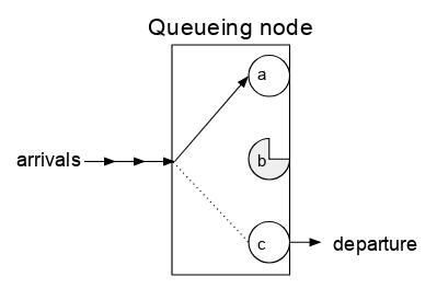
Queuing
A single server follows the first-come, first-served rule and serves clients one at a time from the head of the line. When the service is finished, the customer moves down the line and the system has one less customer.
When adopting this type of queuing model, following assumptions are made:
- Customers are limitless and patient,
- customer arrivals and service rates also follow exponential distributions,
- The waiting line is managed on a first-come, first-served basis.
The likelihood that the waiting area may in fact be constrained is an evident constraint. Another scenario is that the arrival rate varies by state. That example, if they see a big line, potential customers will be deterred from joining it.
Multiple Server model: Multiple service facilities are operating concurrently and provide the same service in a multi-server queue. More than one station can provide service to every customer in the queue. Following poison and exponential distribution are the arrival and service times.

Solved Example: 9134-01
Customers arrive at a reception counter at an average interval rate of 10 minutes and the receptionist takes an average of 6 minutes for one customer. Determine the average queue length.
A. 9/10
B. 7/10
C. 11/10
D. 3/10
Correct Answer: A
Solved Example: 9134-02
The term 'Jockeying' in queuing theory refers to:
A. Not entering the long queue
B. Leaving the queue
C. Shifting from one queue to another parallel queue
D. None of the above
Correct Answer: C
Solved Example: 9134-03
Cars arrive at a service station according to Poisson's distribution with a mean rate of 5 per hour. The service time per car is exponential with a mean of 10 minutes. At steady state, the average waiting time in the queue is:
A. 10 minutes
B. 20 minutes
C. 25 minutes
D. 50 minutes
Correct Answer: D
Solved Example: 9134-04
Queuing theory is associated with:
A. Sales
B. Inspection time
C. Waiting time
D. Production time
Correct Answer: C
Solved Example: 9134-05
Queueing theory deals with problems of:
A. Material handling
B. Reducing the waiting time or idle time
C. Better utilization of man services
D. Effective use of machines
Correct Answer: B
Solved Example: 9134-06
In queuing theory, the nature of the waiting situation can be studied and analysed mathematically if:
A. Complete details of items in, waiting line are known
B. Arrival and waiting times are known and can be grouped to form a waiting line model
C. All variables and constants are known and form a linear equation
D. The laws governing arrivals, service times, and the order in which the arriving units are taken into source are known
Correct Answer: D
Solved Example: 9134-07
The reasons which are basically responsible for the formation of a queue should be that:
A. The average service rate Hess than the average arrival rate
B. Output rate is linearly proportional to input
C. Output rate is constant and the input varies in a random manner
D. All of the above
Correct Answer: D
Solved Example: 9134-08
Monte Carlo solutions in queuing theory are extremely useful in queuing problems:
A. That can't be analysed mathematically
B. Involving multistage queuing
C. To verify mathematical results
D. All of the above
Correct Answer: A
Markov Processes
Learning Objectives:
- Understand the basic concept of Markov Processes as mathematical models for systems with discrete states and probabilistic transitions.
- Define and explain the Markov property, which states that the future behavior of a system depends only on its current state and is independent of past states.
- Create state transition diagrams to visually represent the states, transitions, and associated probabilities of a Markov Process.
- Learn how to construct and use the state transition matrix to describe the probabilities of transitioning between states in a Markov Process.
- Understand and apply techniques for calculating the steady-state probabilities of each state in a Markov Process.
- Define and compute limiting probabilities, which represent the long-term probabilities of being in each state as time approaches infinity.
A Markov process is a random process in which the future is independent of the past, given the present.

Joxemai4, CC BY-SA 3.0, via Wikimedia Commons
Markov Processes are mathematical models used to describe systems that transition from one state to another over time in a probabilistic manner. These processes are widely applied in various fields, including engineering, finance, physics, and computer science.
Key Concepts:
- State: Markov Processes involve a set of states, each representing a possible condition or situation of the system under consideration. These states are discrete and finite.
- Transitions: The system moves from one state to another based on transition probabilities. These probabilities define the likelihood of moving from one state to another in a single time step.
- Markov Property: Markov Processes adhere to the Markov property, which means that the future behavior of the system depends only on its current state. Past states have no influence on future transitions.
State Transition Diagram:
A state transition diagram is a graphical representation of a Markov Process. It consists of nodes (representing states) and arrows (representing transitions) with associated probabilities.
Steady-State Analysis:
Steady-state analysis involves finding the long-term probabilities of the system being in each state. This is typically done by solving a set of linear equations or using iterative methods.
Limiting Probabilities:
Limiting probabilities represent the long-term probabilities of being in each state as time approaches infinity. They are obtained by studying the behavior of the system over a large number of transitions.
Applications:
Markov Processes find applications in various domains:- Telecommunications: Modeling network traffic and call routing.
- Finance: Assessing investment strategies and stock price movements.
- Quality Control: Analyzing the reliability and maintenance of systems.
- Epidemiology: Modeling disease spread and healthcare planning.
Time Homogeneous vs. Time Inhomogeneous:
In time-homogeneous Markov Processes, transition probabilities remain constant over time. In contrast, time-inhomogeneous processes allow transition probabilities to vary with time.
Ergodicity:
An ergodic Markov Process is one in which, over time, the system will visit all states with nonzero probability. This property is essential in analyzing long-term behavior.
Markov Chain Monte Carlo (MCMC):
Markov Chains, a specific type of Markov Process, are used in MCMC simulations to approximate complex mathematical problems, such as Bayesian inference and optimization.
In summary, Markov Processes are powerful tools for modeling and analyzing systems with probabilistic transitions. They are used to gain insights into the behavior of systems over time, including steady-state probabilities and limiting behaviors. A solid understanding of Markov Processes is valuable for engineers and professionals in various fields, as it enables them to make informed decisions and predictions in the face of uncertainty.
Solved Example: 9135-01
The probability density function of a Markov process is:
A. p(x1,x2,x3.......xn) = p(x1)p(x2/x1)p(x3/x2).......p(xn/xn-1)
B. p(x1,x2,x3.......xn) = p(x1)p(x1/x2)p(x2/x3).......p(xn-1/xn)
C. p(x1,x2,x3......xn) = p(x1)p(x2)p(x3).......p(xn)
D. p(x1,x2,x3......xn) = p(x1)p(x2 *x1)p(x3*x2)........p(xn*xn-1)
Correct Answer: A
Inverse Probability Functions
- The Inverse Function “undoes” what the function does.
- The Inverse Function of the BLUE dye is bleach. The Bleach will “undye” the blue egg and make it white. In the same way, the inverse of a given function will “undo” what the original function did.